Mario games are fun and challenging. Nintendo has been spending a great deal of effect to design and implement them. In 2015, they released Super Mario Maker. The community could finally legally make and share their levels. With their creativity and dedication, many fun levels which Nintendo would not make were born. Unsurprisingly, the community also made loads of trash levels. Some were only by-products of learning to be great level makers, but the others were purposely built to torment players. In 2019, Nintendo released a sequel to the game Super Mario Marker 2. There has been a new game mode, endless challenge.
No-skip Endless Challenge
In the endless challenge, you try to complete as many levels the game throws at you as possible. You pick a difficulty and have a certain number of lives to begin. For expert difficulty, you have 15 lives at the start.
| Difficulty | Number of Starting Lives |
|---|---|
| Easy | 5 |
| Normal | 5 |
| Expert | 15 |
| Super Expert | 30 |
Each time you die on a level, you lose a life. When you have no remaining lives, the run ends. There are multiple ways to gain lives, but you can only redeem them after clearing a level. If there is a flagpole at the end of a level and you touch the top, you receive a life. Similar to other Mario games, collecting a green mushroom or 100 coins grant you a life too. Besides, you can stomp on multiple enemies without touching the ground or using a shell to kill them consecutively to gain lives as well. You can only redeem as most 3 lives in a level because the game limit that to prevent you to farm lives. A generous level maker will unconditionally give you 3 lives or loads of coins. Conversely, an inexperienced or mean one will give you nothing and even block you from reaching the top of the flagpole to gain a life. In addition to the life gain limit in a level, you can have maximally 99 lives.
The game randomly chooses a level made by the community according to the difficulty as your next level. The exact formula of how the game determines the difficulty of a level is not publically known. It is however strongly correlated to the level clear rate ($ \frac{\text{#clears}}{\text{#trials}} $), player clear rate ($ \frac{\text{#winning players}}{\text{#trying players}} $), and the level maker's number of upload trials. For expert difficulty, you should expect to occasionally encounter a level with a clear rate as low as 2%. For such a level, the community wins 1 out of 50 trials. Very rarely, you will encounter a level with a difficulty like the super expert because the formula does not rate the level accurately enough. It seems to happen more often on new levels which have more uncertainty.
The game allows you to skip levels so you will have a more enjoyable experience in the endless challenge. Your run will not immediately end because you encounter a level poorly made, requiring some skills or knowledge you do not have. However, what hardcore gamers want is the exact opposite. Skipping makes the challenge too easy, so they handicap themselves by forbidding it.
Your life gain on each level needs to be at least on par with your loss on average to keep a run going in the long term. If you are an average player having only a clear rate of a few percent on an expert level, you virtually have no hope of passing 1000 levels, not even 10 levels. Besides a high clear rate, you also need a lower variance in your life change so you can resist a longer streak of bad levels.
Theory
The most reliable and straightforward way to estimate the difficulty of the no-skip endless challenge is to use an average success rate of many runs. It is the same as estimating the fairness of a coin. We can use the binomial proportion to obtain the uncertainty in terms of the confidence interval. A confidence interval is an interval that covers the true parameter with a certain amount of long-run frequency for (hypothetically) repeatedly random sampling. The sampling process works well for poorly performed players whose success rates are close to 0 because their runs do not last long. It is not the case for skilled players. A run may take many hours. For example, with an average of 3 minutes per level, a successful run will take 50 hours to complete. Without many runs, the uncertainty is large, so the overall confidence intervals are too. For example, the 99% confidence interval of a win and a loss is [6.2%, 93.8%]. Therefore, It is worth putting efforts to squeeze out more information from the existing data to shrink the uncertainty. We will model the problem as a Markov process and use the bootstrap to infer the success rate and the confidence intervals. Generally, the estimated success rate should be closer to the true value for all possible true values and samples. Similarly, the overall confidence intervals should be tighter.
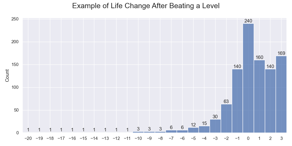
An example of life changes after beating each of the 1000 levels. The sample success rate is about 50%.
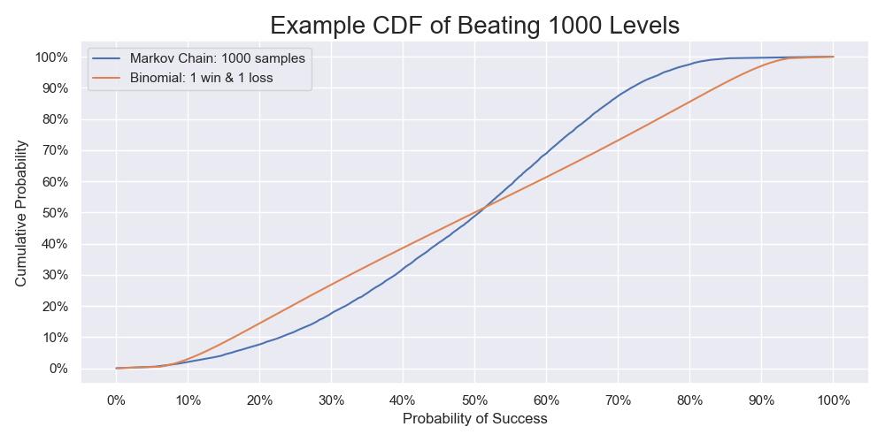
The cumulative probability functions calculated by the two methods. The one calculated by modeling the problem as a Markov process and using the bootstrap is based on the distribution of the life changes above. The other one calculated by the binomial proportion is based on one win and one loss.
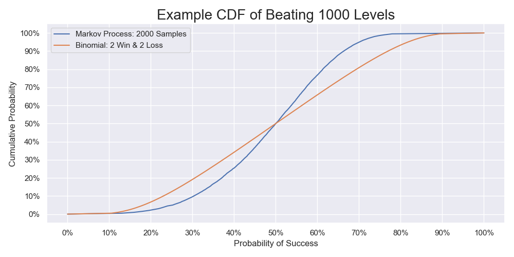
The cumulative probability functions calculated by the two methods with doubling the samples. The one calculated by modeling the problem as a Markov process and using the bootstrap is based on doubling the distribution of the life changes above. The other one calculated by the binomial proportion is based on two wins and two losses.
We begin by identifying the essence of the process. At the start of a run, a player has 15 lives. The game randomly draws a level as the next level. After playing a level, the number of life may change with an amount ranging from losing all their lives to gaining 3 lives. If the player loses all their lives, the run ends. If the player loses all their lives, the run ends. Conversely, if they gain so many lives that the total exceeds 99, it will still be 99. The number of life and the change are sufficient to describe the player state and a level, respectively.
Because of the game being closed source, Nintendo not publishing any detail, and insufficient samples, we need to make a few assumptions and simplifications:
- The game draws a level independent of the number of lives.
- The game draws a level independent of the completed levels.
- The player's performance is independent of the previous levels.
- The player performs practically the same when their number of lives is from 1 to 96 or 97 to 99.
- The difficulty of the levels is approximately the same across different runs.
There has been no information about the independence in the first assumption. Considering that it seems to be and tight budgets are common in the game industry, it is reasonable to assume that Nintendo chose the simplest implementation. The second assumption is at least a close approximation of the real mechanism. There are 20 million levels1 as of September 2020. Even if a small subset has the expert difficulty, there should still be enough levels that drawing 1000 levels with replacements is approximately the same as drawing without replacements. Thus, we do not need to worry about which case it is. We can simply model it as drawing with replacements. The remaining assumptions are to reduce the sample requirements. Otherwise, we will need a more sophisticated model or much more samples. Careful analysis may disproof some of the assumptions, but it is out of the scope of this article. Regardless, the following will at least serve as an entry point for more sophisticated analysis even if you do not agree with the assumptions.
Modelling as a Markov Process
An easy way of determining the probability is to simulate many runs. Such a simulation can run 500 times per second on my computer. However, because the variance of the runs is very high, the success rate needs 1 million runs to start converging. If all we need is the expected success rate, it is acceptable to let it run for 33 minutes. But we cannot ignore the potentially significant uncertainty in the collected statistics. We can simulate the sampling process and run the 1 million simulations many times, say 1,000, to approximate the uncertainty. That alone will take 23 days of computational time. To ensure that 1,000 simulations are enough, we should repeat it many times too, say 1,000 times, to verify it. The approach quickly becomes impractical if we want to be thorough. Instead, if we model the problem as a Markov process, we can calculate the success rates analytically 2,500 times per second, not once per 33 minutes. Since the solutions are exact, we eliminate the uncertainty in the simulation.
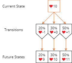
A Markov process is a random process in which the current state determines the future state. In our case, the player's number of lives is the state. By knowing the probability of different life changes after completing a level, we can predict the probabilities of the future number of lives. For example, suppose that a player currently has 10 lives. The probabilities of -1 life, +0 life, and +1 life after finishing the next level are 20%, 30%, and 50%, respectively. The probabilities of having 9, 10, and 11 lives after finishing the next level are 20%, 30%, and 50%, respectively.
The probabilities of the future state can be calculated by considering each mututally exclusive branch separately.
Furthermore, different numbers of lives are mutually exclusive states, and so do life changes as mutually exclusive events. By the law of total probability, we can separately consider different states then sum the probabilities for all the outcomes. Referring to the example above but now the probabilities of the current state having 9 and 10 lives are 40% and 60%, respectively, the probability of having 9 lives after finishing the next level is
$$ \begin{aligned} P_\text{next}(\textcolor{red}{♥}=9) ={} & P_\text{current}(\textcolor{red}{♥}=9) \times P(\Delta\textcolor{red}{♥}=0) \\ & + P_\text{current}(\textcolor{red}{♥}=10) \times P(\Delta\textcolor{red}{♥}=-1) \\ ={} & 40\% \times 30\% + 60\% \times 20\% \\ ={} & 24\% \end{aligned} $$Similarly, the probabilities for 8, 10, and 11 lives are 8%, 38%, and 30%, respectively.
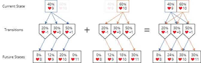
The probability of a future state can be calculated separately then summed.
It is more convenient to organize the calculation in the following matrix form. In addition, the matrix form allows us to leverage accelerated processings by computers during bootstrapping.
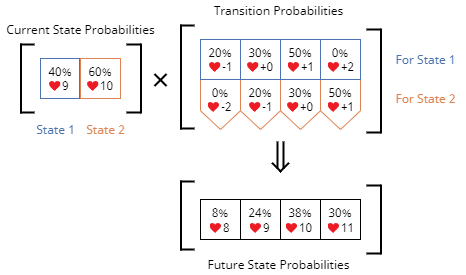
The calculation in the matrix form.
For the actual problem, let
- $ s_k $ be a 100-dimensional row vector for the states after finishing $ k $ levels,
- $ P_s(k,\textcolor{red}{♥}=n) $ be the probability of the state after finishing $ k \in \set{0,1,2,\ldots} $ levels and having $ n \in \set{0,1,2,\ldots,99} $ lives,
- $ T $ be a 100×100 right stochastic matrix,
- $ P_t(\textcolor{red}{♥}=n,\Delta\textcolor{red}{♥}=m) $ be the probability of transiting from having $ n $ lives to $ (n+m) \in \set{0,1,2,\ldots,99} $ lives.
The first row in $ T $ is a twist. It allows us to continue to apply the transition to the state even after a run end. This row represents how the absorbing state $ \textcolor{red}{♥}=0 $ is stuck there.
The other rows in $ T $ are mostly some offset versions of the general life change probabilities. Generally, they are the same as the corresponding transition probabilities for each state, i.e., $ P_t(\textcolor{red}{♥}=n,\Delta\textcolor{red}{♥}=m)=P(\Delta\textcolor{red}{♥}=m) $ where $ P(\Delta\textcolor{red}{♥}=m) $ is the probability of life change of $ m \in \set{0,1,2,\ldots,99} $ without considering the minimum (0) and maximum (99) numbers of lives. However, the transition probabilities for 0 lives ought to include the life change probabilities causing the number to drop below 0 and vice versa for 99 lives.
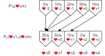
In this example, the life change probabilities are for ranging from -3 lives to +1 life. The transition probabilties for the state having 1 life to the state having 0 lives are the sum of the -3, -2 and -1 life probability.
Formally, the transition probabilities are
$$ \begin{aligned} P_t(\textcolor{red}{♥}=n,\Delta\textcolor{red}{♥}=m) = \begin{dcases} \sum_{q=-\infty}^{m} P(\Delta\textcolor{red}{♥}=q),& \text{if } n+m=0\\ \sum_{q=m}^{\infty} P(\Delta\textcolor{red}{♥}=q),& \text{if } n+m=99\\ P(\Delta\textcolor{red}{♥}=m), & \text{otherwise} \end{dcases} \end{aligned} $$Starting from the initial state that is 100%, by applying the state change repeatedly, we have the probabilities of the state after finishing any number of levels.
$$ \begin{aligned} s_k &= s_0T^k \end{aligned} $$We can then calculate the probability of clearing a certain number of levels, and so that of beating the challenge. The probability of beating $ k $ levels is
$$ \begin{aligned} P(k) &= 1 - P_s(k,\textcolor{red}{♥}=0) \\ &= \sum_{\textcolor{red}{♥}=1}^{99} P_s(k,\textcolor{red}{♥}) \end{aligned} $$Uncertainty Estimation by Bootstrapping
Sampling the frequencies of different life changes allows us to infer the population, the true probabilities of life changes, and then the parameter, the success rate. It is impossible to know the exact values because it requires the player to play every level infinitely many times to measure the frequencies of different life changes. When we only observe a finite number of samples, there is a random variation between the sample and the population. It is crucial to know the possible variations. Otherwise, we do not know how much the estimation is off. In this article, we will go with the frequentist inference. For some simple and common problems, there are formulae to calculate the variations in terms of confidence intervals. However, there seems to be none for this problem. We will use a simulation approach instead.
Bootstrapping is a resampling method based on Monte Carlo simulation. The core idea is very simple but yet powerful. We mimic the sampling process of the population by resampling the sample. The sample becomes a known population. With many resamples, our desired statistic, the sample success rate, forms a distribution that we can compare with the sample. The information allows us to infer the uncertainty in sampling the original population.
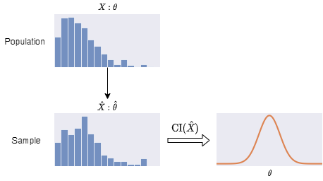
Usually, we can infer the confidence interval of our interested statistic $ \hat{\theta} $ of our samples $ \hat{X} $ using known formulae.
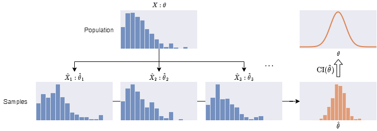
When there are no known formulae, a simple way to study the uncertainty is to repeat the sampling process many times. It trades the reduction of uncertainty with the knowledge in uncertainty.
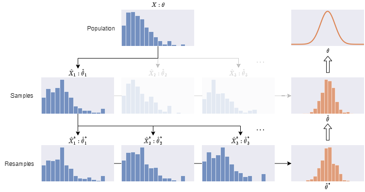
Resampling the only set of observed samples $ \hat{X}^*_1 $ to infer the uncertainty in $ \hat{\theta_1} $ is much cheaper. We can resample $ \hat{X_1} $ many more times than sampling $ X $. It allows us to have the knowledge in uncertainty without sacrificing a smaller uncertainty.
For simplicity, we will use a non-parameteric bootstrap to estimate some confidence intervals of the success rate. It will directly resample the observed samples. There are many popular non-parameteric bootstraps to choose from, basic (aka empirical/reverse percentile), bootstrap-t (studentized basic), percentile, bias-corrected (BC), and bias-corrected and accelerated (BCa). They have different assumptions, so they work in different situations2. The basic bootstrap is based on $ \hat{\theta} - \theta $ and requires it to be pivotal. A pivot is a quantity that is independent of any parameters. It is like a normalized value. The bootstrap-t uses $ \frac{\hat{\theta} - \theta}{\hat{\sigma}} $ instead so it allows variation in the variance. On the contrary, the percentile bootstrap directly works on $ \hat{\theta} $. It only requires existence of a monotonically increasing function $ g $ such that $ \hat{w} = g(\hat{\theta}) - g(\theta) $ is a normal distribution of 0 mean. The amazing and magical part is that you do not need to provide $ g $ at all. The BC bootstrap extends the percentile bootstrap by supporting bias in $ \hat{w} $. Furthermore, the BCa bootstrap supports bias and skewness in $ \hat{w} $. If you are interested in the theory behind it, I would recommend you to read the section "BOOTSTRAP CONFIDENCE INTERVALS" in Bootstrap confidence intervals: when, which, what? A practical guide for medical statisticians by James Carpenter and John Bithell2.
To make non-parametric bootstraps compatible with the way we calculate the transition probabilities, we will simply throw away samples of levels starting with 97 to 99 lives this time. The levels limit the maximum life change. This condition is called right censoring. For example, consider a level that starts with 97 lives and ends with 99 lives. The life change is +2. When applying the life change to a level that starts with 1 life, we do not know if it should end with 3 or 4 lives. A more advanced way to calculate the transition probabilities is to incorporate all levels into a distribution, but it requires the usage of parametric bootstraps. I will leave it for a future article.
It is unclear if any one of the bootstraps above will work. We will conduct a simluation study of the coverages of the confidence intervals along the way. Using the same resampling technique, we can empirically test the coverages of the confidence intervals. The sample becomes a population, and this time we resample it to simulate the original sampling process. For each resample, we use the bootstraps to calculate the confidence intervals. Because we know the population, and so does the true success rate, we can count the number of instances in which the confidence intervals cover the true success rate. As a result, we can compare the cover rate with the desired rate to determine if the bootstraps work.
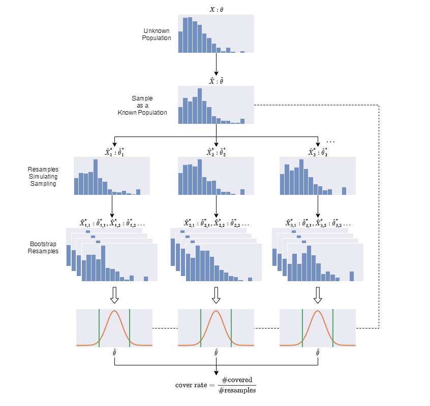
An illustration of the procedure of the study of the coverages. The sample acts as a population. It is resampled to mimic the original sampling process. A confidence interval is calculated using the bootstrap for each set of resamples. Counting the number of confidence intervals that cover the statistic of the sample gives the actual coverage. It should be within random variations of the nominal coverage.
Data Collection
We will study the winning probability of one of the most skilled players in Super Mario Marker 2, PangaeaPanga (aka Panga). His playthrough videos are available on his YouTube playlist will provide us the data. First, we will need to gather the numbers of different life changes. Instead of tediously recording every event manually, we will use computer vision to automate it. We will identify frames containing the number of lives after the completion of each level, recognize the texts, and save them into a list.
Frame Detection
We start by analyzing the information in the videos. Conveniently, Panga put his number of completed levels on the top right corner. He also showed all the level title scenes, which contained the number of lives. A simple handcrafted detector is more than enough for the job.
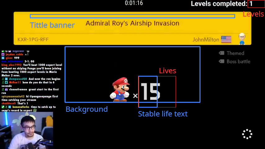
An example of the title scene. The blue and red bounding boxes show the features and the information to extract respectively.
The title scenes are easily recognizable by a huge yellow box at the top and a black background. We pick some coordinates for the bounding boxes to count the pixels matching our targeted colors. The average colors will not work as our thresholds because the videos are encoded by lossy compression. The colors are distorted and differ at different locations and times. There are no other kinds of frames similar to this, so we can use some generous thresholds without worrying about much false detection of frames. We should be careful that not all the frames are as clean as the example above. Sometimes, there are emotes (icons) flying around and text overlays. We should use some smaller thresholds for the number of pixels.
Using the first detected frame of each title scene to read the number of lives will give a poor result. The text showing the number of lives has a popup animation that enlarges from the bottom left. The text is too small at the beginning of the animation. To work around it, we wait for a larger text by counting the number of white pixels within the bounding box enclosing the widest left digit, 8. The threshold should be small enough to accommodate the thinnest digit, 1.
We will refine the thresholds by examining the failure cases by running the program a couple of times after implementing the text recognition in the next step. Below is a peek of the final thresholds:
| Feature | Color | Lower Threshold | Upper Threshold | Area |
|---|---|---|---|---|
| Tittle banner | ■ #FBCB03 | ■ #E6BE00 | ■ #FFDC14 | >70% |
| Background | ■ #000000 | ■ #000000 | ■ #060606 | >70% |
| Stable life text | ■ #FFFFFF | ■ #C8C8C8 | ■ #FFFFFF | >14% |
The source code is available in the GitHub repository of this site. I will not show it and explain the implementation here. There are plenty of tutorials on fundamental computer vision on the Internet.
Optical Character Recognition
After locating the frames, the next step is to recognize the text corresponding to the number of lives and completed levels. There are many ways to do it. Simple template matching provided by OpenCV should work, but we will use Tesseract instead. Tesseract comes with pre-trained models, so we do not need to prepare any templates to match or train. Unfortunately, whitelisting the built-in pre-trained English model with digits just happens to perform poorly. It is probably because the architecture of the neural network does not handle whitelists well. Before trying to train a specialized model using the numbers from the frames or switching to template matching, we should try other pre-trained models first. A Tesseract contributor, Shreeshrii, shared their refined models in his GitHub repository. digits.traineddata works much better than the built-in English model.
Data Cleansing
After implementing the process, we get the level information that requires some data cleansing. We should not blindly accept the output as there may be errors in the output. Panga gave up several times which he had rough starts. Besides, there may be recognition errors. An easy way to spot major errors is to check for invalid level changes and life changes. Generally, each consecutive level should have +1 level change and less than or equal to +3 life change. For smaller incorrect life changes, the only way to eliminate them is to manually compare the output against the videos. We will skip it and assume that they are insignificant to the estimated success rate.
There are only 12 erroneous levels out of 1058 levels. The error rate is 1.13%. At this point, it does not worth the time to improve the frame detector and text recognition. We should manually fix those errors.
Simulation
Before proceeding to the calculation, we need to filter out levels starting with 97 to 99 lives. There are 726 remaining levels that we can use. He gained lives 52.5% of the time, lost lives 26.6% of the time, and neither 20.9% of the time. On average, he gained 0.233 lives after playing a level. The distribution is as follow:
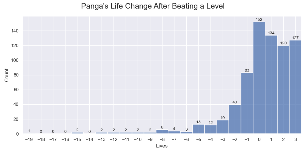
Panga's performance on the 726 levels.
Sample Success Rate
Now we can calculate Panga's sample success rate of beating the challenge by applying the theory of Markov process. The calculation is also a building block in the bootstrap for calculating the confidence interval. The sample probability is 61.6%.
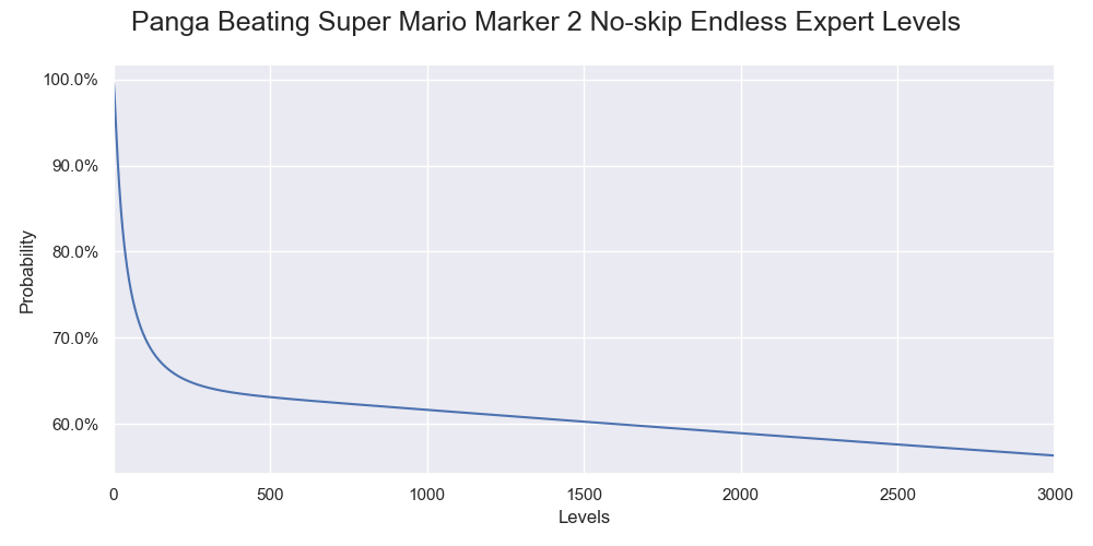
The estimated probability of Panga beating various numbers of levels in the endless challenge without skipping.
Bootstrap
We will use the bootstrap module in Arch to calculate the confidence interval. I choose it instead of SciPy because it is easier to experiment with. It provides more bootstrap methods and natively supports resuing the results when changing bootstrap methods.
Simulation Study of Coverages
Recall of the procedure of testing the coverage.
If you use Arch directly, you will encounter the following exception
Empirical probability used in bias correction is 0 or 1, and so bias cannot be corrected. This may occur in extremum statistics that are not well approximated by a normal in a finite sample.
For us, it happens when a simulated sample $ \hat{X}_r^* $ excludes all occurrences of -15 lives and below. The maximum life loss is 14, so the survival probability of the first level is 100% for all the bootstrap resamples $ \hat{X}_{r,s}^* $. Patching Arch to handle the problem is fairly easy and fast.
We start by preliminarily checking the coverages of 95% confidence interval for several common bootstrap methods, basic, percentile, bias-corrected (BC), and bias-corrected and accelerated (BCa). 1000 bootstrap resamples repeating 1000 times is enough. It means that there are 1000 simulated samples $ \hat{X}_r^* $ and 1000 bootstrap resamples $ \hat{X}_{r,s}^* $ for each simulated samples. After obtaining a confidence interval for each of the 1000 true success rate $ \hat{\theta} $, we count numbers of confidence intervals that contain their corresponding success rate. I ran the test for levels from 1 to 3000 and plotted the graph below.
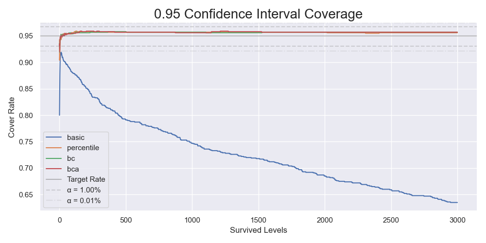
The coverages of the 95% confidence intervals for 1000 bootstrap resamples repeating 1000 times.
The dotted lines in the graph show the thresholds rejecting the null hypotheses that the corresponding measured coverages were the same as the nominal coverage of 95%. It was clear that the basic bootstrap gave different coverages. On the contrary, we could not reject the null hypotheses for the percentile, the BC, and the BCa bootstrap. You should be cautious that it did not mean that the coverages were the same as the nominal coverage. It is impossible to prove these null hypotheses. To tell if those methods gave the "same" coverages as the nominal coverage, we should perform equivalence tests. From now on, we will exclude the basic bootstrap and increase the number of resamples and repeats.
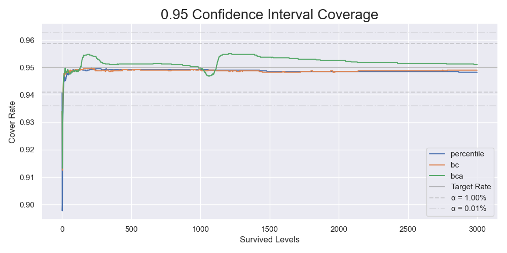
The coverages of the 95% confidence intervals for 40000 bootstrap resamples repeating 4000 times.
| Levels | Percentile | BC | BCa |
|---|---|---|---|
| 1000 | 94.9% | 94.9% | 95.0% |
| 2000 | 94.8% | 94.8% | 95.2% |
| 3000 | 94.8% | 94.9% | 95.1% |
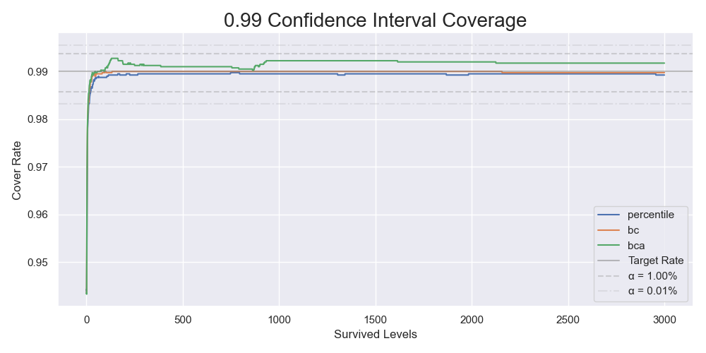
The coverages of the 99% confidence intervals for 40000 bootstrap resamples repeating 4000 times.
| Levels | Percentile | BC | BCa |
|---|---|---|---|
| 1000 | 99.0% | 99.0% | 99.2% |
| 2000 | 99.0% | 99.0% | 99.2% |
| 3000 | 98.9% | 99.0% | 99.2% |
They all performed similarly. I will not perform the equivalence tests here. Let us assume that they are equivalent to our use. We will use the BCa for the analysis.
Result
Combining the sample probability with the bootstrap result using the BCa for 40000 resamples gave the following result. As a bonus, I calculated all the probabilities for levels up to 3000. You should keep in mind that the probabilities of the confidence intervals shown below refer to the long-run frequencies of covering the true success rates for (hypothetical) repeated random sampling. A particular confidence interval either covers or does not cover the true success rate. After getting a sample and revealing the confidence interval, the cover rate of the confidence interval is only epistemic (one's ignorance). Further interpretations require a deeper understanding of the properties of bootstrapping. The definition of confidence intervals is loose in which it only concerns the cover rate. Some procedures give opposite widths or counter-intuitive intervals. Richard D. Morey, Rink Hoekstra, Jeffrey N. Rouder, Michael D. Lee, and Eric-Jan Wagenmakers explained the issues nicely in The fallacy of placing confidence in confidence intervals3. Below is the result:
| Levels | Probability | 95% CI | 99% CI |
|---|---|---|---|
| 1000 | 61.6% | [15.7%, 85.4%] | [5.84%, 89.4%] |
| 2000 | 58.9% | [8.38%, 86%] | [1.78%, 90.2%] |
| 3000 | 56.3% | [3.96%, 86%] | [0.43%, 90.1%] |
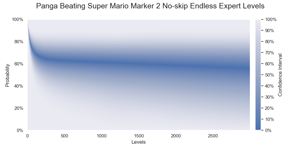
Probabilities of Panga successfully beating various numbers of levels. The darkest color denotes the medians of the probabilities.
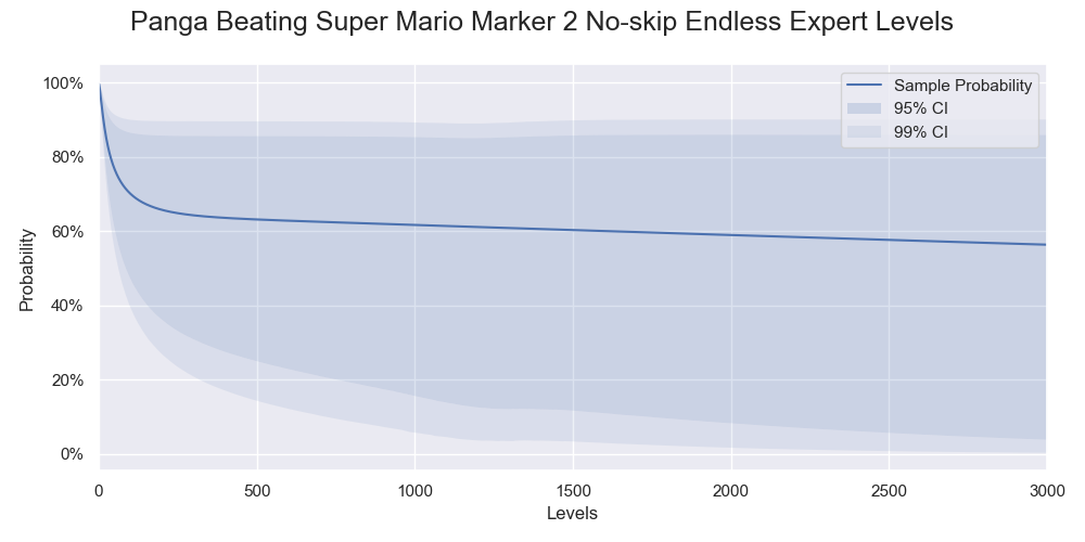
Probabilities of Panga successfully beating various numbers of levels. Only 95% and 99% confidence intervals are shown.
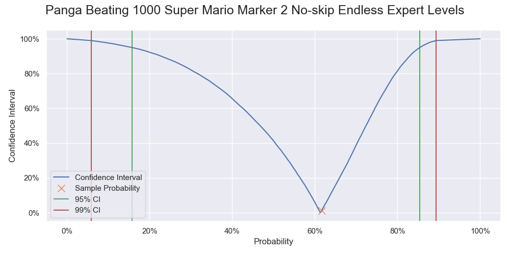
Probability of Panga successfully beating 1000 levels. It is a vertical slice of the level 1000 of the previous two graphs, and like a graph of the cumulative probability but with the 0% - 50% part being flipped upward.
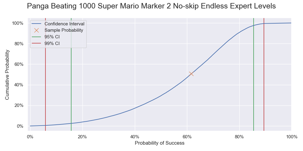
Cumulative probability of Panga successfully beating 1000 levels.
Conclusion
Undoubtedly, beating 1000 endless expert levels without skipping in Super Mario Marker 2 is hard for most players. It is not for ones without top-notch skills and strong determination. This article has quantified the difficulty by using the theory of the Markov process, bootstrapping, and one of the best players' data. You are likely to have even more questions about this challenge other than the success rate. In the future, we will delve deeper into the details in part 2.
A tweet by Nintendo of America on 4 Sep, 2020. https://twitter.com/NintendoAmerica/status/1301928016004644864 ↩︎
Carpenter, J. and Bithell, J. (2000), Bootstrap confidence intervals: when, which, what? A practical guide for medical statisticians. Statist. Med., 19: 1141-1164. https://doi.org/10.1002/(SICI)1097-0258(20000515)19:9<1141::AID-SIM479>3.0.CO;2-F ↩︎
Morey, R.D., Hoekstra, R., Rouder, J.N. et al. The fallacy of placing confidence in confidence intervals. Psychon Bull Rev 23, 103–123 (2016). https://doi.org/10.3758/s13423-015-0947-8 ↩︎