In part 1, we learned how to use bootstraps to calculate confidence intervals of Panga's success rates of beating the various numbers of levels without skipping. We threw away the censored samples that were 31% of the samples for simplicity. This time, we will use all of them to infer the success rates and confidence intervals.
A Better Estimator
The maximum number of lives, 99, limits the maximum life change after beating a level in addition to the maximum 3-life gain. For a player having a starting life from 1 to 96 before playing a level, there is no censorship in the observation of their life change after beating the level. However, if they have a starting life from 97 to 99, the observed life change is capped. When mixing these samples with the former samples, we need to take care of this right censoring problem.
The Kaplan–Meier estimator is our solution. We will group the probabilities of life changes that the censoring does not skew the estimation. By applying the same technique to each group containing multiple life changes and ignoring the censored samples useless to the subgroups, we will be able to estimate the probabilities of each subgroup. Repeating the steps will eventually give us the probabilities of each life change.
Because we are dealing with a right censoring, we will estimate the probabilities from the most life loss toward the most life gain. For life losses, we will simply count the proportion for each one and group the remaining for life gain greater than or equal to 0. Doing so will allow us to include the censored samples when estimating the probabilities of each group. After throwing away the samples with 99 starting lives and negative life changes, we will count the proportion for 0-life change and group the remaining for 1 or more life gain. The overall proportion for 0-life change will be the product of the previous proportion for 0 or more life gain and the current proportion for 0-life change. By repeating a similar procedure for 1 to 3-life gains, we will get the probabilities for all life changes using all the samples.
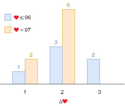
For example, a player having 97 starting lives gained 1 life once and 2 lives 6 times. In part 1, we threw away these censored samples and only relied on the samples with 1 to 96 starting lives.
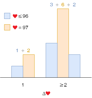
To calculate the probability of 1-life gain, we group the samples into 1-life gain and other life gains. It is the former divided by the sum of both, which is $ \frac{1 + 2}{1 + 2 + 3 + 6 + 2} = 21\%$. That of 2 or more life gain is $ 100\% - 21\% = 79\% $
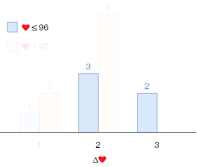
Then we throw away the samples with 97 start lives and 1-life gain. The probabilty of 2-life gain is $ \frac{3}{3 + 5} \times 79\% = 30\% $. That of 3-life gain is $ 79\% - 30\% = 49\% $.
Formally, let
- $ \textcolor{red}{♥} \in \set{0,1,2,\ldots,99} $ be the number of starting lives.
- $ \Delta\textcolor{red}{♥} \in \set{-99, -98, -97, \ldots, 3} $ be the life change.
- $ X(c) $ be the number of samples that condition $ c $ is true.
- $ P(\Delta\textcolor{red}{♥}) $ be the probability of life change of $ \Delta\textcolor{red}{♥} $ without considering the censoring.
The probabilities of negative life changes, $ m $, are:
$$ \begin{aligned} P(\Delta\textcolor{red}{♥}=m) &= \frac{X(1\le\textcolor{red}{♥}\le99,\Delta\textcolor{red}{♥}=m)}{X(1\le\textcolor{red}{♥}\le99,-99\le\Delta\textcolor{red}{♥}\le3)}, & -99 \le m < 0 \end{aligned} $$The probability of all non-negative life changes is the complement:
$$ P(\Delta\textcolor{red}{♥}\ge 0) = 1 - P(\Delta\textcolor{red}{♥}<0) $$The probability of 0-life change is:
$$ P(\Delta\textcolor{red}{♥}=0) = P(\Delta\textcolor{red}{♥}\ge 0) \frac{X(1\le\textcolor{red}{♥}\le98,\Delta\textcolor{red}{♥}=0)}{X(1\le\textcolor{red}{♥}\le98,0\le\Delta\textcolor{red}{♥}\le3)} $$The probability of 1 or more life changes is:
$$ P(\Delta\textcolor{red}{♥}\ge 1) = P(\Delta\textcolor{red}{♥}\ge0) - P(\Delta\textcolor{red}{♥}=0) $$Repeating the same logic gives the remaining probabilities:
$$ \begin{aligned} P(\Delta\textcolor{red}{♥}\ge 1) &= P(\Delta\textcolor{red}{♥}\ge0) - P(\Delta\textcolor{red}{♥}=0) \\ P(\Delta\textcolor{red}{♥}=1) &= P(\Delta\textcolor{red}{♥}\ge 1) \frac{X(1\le\textcolor{red}{♥}\le97,\Delta\textcolor{red}{♥}=1)}{X(1\le\textcolor{red}{♥}\le97,1\le\Delta\textcolor{red}{♥}\le3)} \\ P(\Delta\textcolor{red}{♥}\ge 2) &= P(\Delta\textcolor{red}{♥}\ge1) - P(\Delta\textcolor{red}{♥}=1) \\ P(\Delta\textcolor{red}{♥}=2) &= P(\Delta\textcolor{red}{♥}\ge 2) \frac{X(1\le\textcolor{red}{♥}\le96,\Delta\textcolor{red}{♥}=2)}{X(1\le\textcolor{red}{♥}\le96,2\le\Delta\textcolor{red}{♥}\le3)} \\ P(\Delta\textcolor{red}{♥}=3) &= P(\Delta\textcolor{red}{♥}\ge2) - P(\Delta\textcolor{red}{♥}=2) \\ \end{aligned} $$Sampling Process
The sampling process is different from independently drawing samples from a distribution with replacements that non-parametric bootstraps work perfectly. The censoring of a sample depends on the starting life where the life is the sum of the starting lives and the life change of its predecessor. The probabilities of life changes correlate with the censoring. The better the player is, the heavier the censoring there is. It is not obvious if a simple non-parametric bootstrap will work. Instead, we use parametric bootstraps with a model of the sampling process to calculate the confidence intervals.
Like the non-parametric counterparts, the BCa version is the least restrictive and generally provides the most accurate confidence intervals. However, it is more complicated than the non-parametric counterpart, especially when dealing with correlated samples. The details can be found in section 4 of The Automatic Construction of Bootstrap Confidence Intervals by Bradley Efron and Balasubramanian Narasimhan1.
Rather than jumping into another deep rabbit hole immediately, we will spend some time studying the problem first by examining the actual differences between the samples obtained by different sampling processes. Below are some simulations of the original sampling, a multinomial sampling, and a non-parametric resampling process. Including the resampling process will help us to decide if a BCa bootstrap is necessary. There were 1058 samples of levels from part 1. The life change probabilities given by the Kaplan-Meier estimator formed a multinomial distribution. It was the basis of the simulations for the original sampling and multinomial sampling.
The original sampling process drew a sequence of 1058 levels from the distribution with replacements. It assigned 15 starting lives to the first level. The starting lives for each successive level were the sum of the current start lives and the life change. They were less than or equal to 99. Whenever a starting life fell below 1, it became 15 as if a run restarted. The Kaplan–Meier estimator gave an estimate of the life change probabilities for a new set of samples. In the simulation, I repeated the process 1,000,000 times and obtained distributions of the simulated estimates.
In the multinomial sampling, drawing 1058 levels was the whole process. There was no censoring. The process was simple enough that a formula for the exact distributions existed. I did not have to run a simulation.
The resampling was the same as those in non-parametric bootstraps. It directly drew new sets of 1058 samples from the 1058 samples with replacements. Like the other simulation, I repeated it 1,000,000 times and obtained the corresponding distributions again.
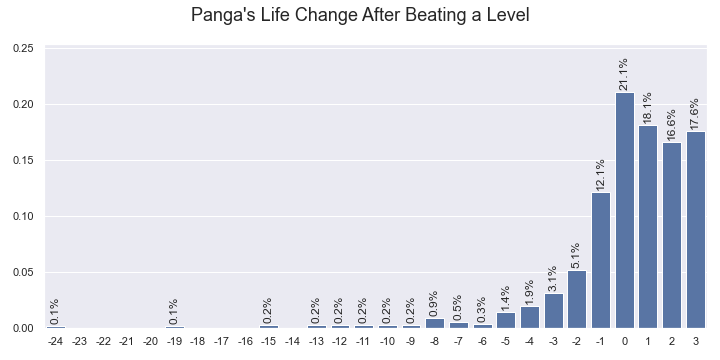
The probabilties of Panga's life change after beating a level estimated by the Kaplan–Meier estimator.
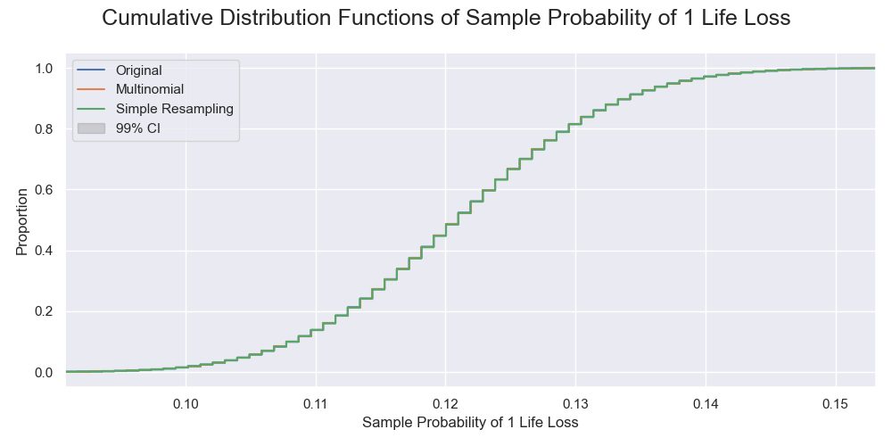
The cumulative distributions of the probabilities of 1 life loss by the simulated sampling processes. The censoring did not affect life loss, so the distributions were the same.
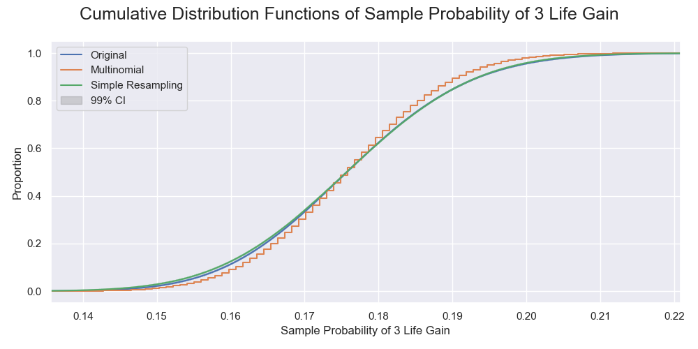
The cumulative distributions of the probabilities of 3-life gain by the simulated sampling processes. That by the original sampling and the resampling were very close, unlike the multinomial sampling.
The distributions of the probabilities of the non-negative life changes calculated by the original sampling process and the resamplings were considerably close. You would probably guess that the distributions of the sample success rates would behave the same. Simulating 400,000 times gave the following results. That by the resampling was indeed very close to that by the original sampling, but that by the multinomial sampling was even closer. Using only certain numbers of initial samples, e.g., 25% or 50%, gave similar results. A rigorous proof should cover all distributions of life change probabilities, but for now, let us assume that all sampling processes are practically the same.
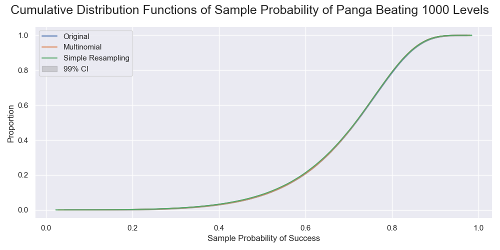
The cumulative distributions of the success rates of beating 1000 levels. The line for the original sample was behind that for the multinomial sampling. All were very close. There was only a small bias in that by the resampling.
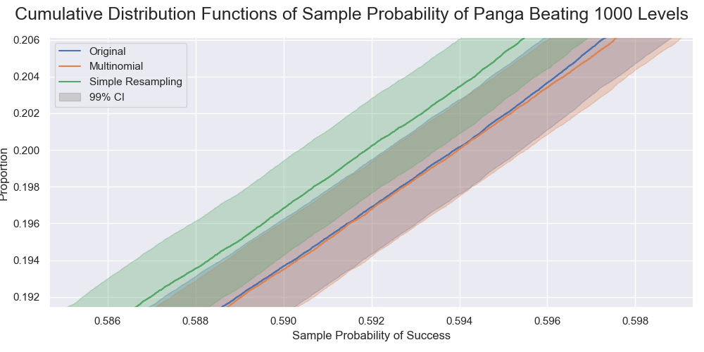
A zoomed section of the previous graph. The distributions by the original sampling and the multinomial sampling were virtually indistinguishable. That by the resampling was slightly different but still practically the same.
Bootstrap Method
If you pay close attention to the result in part 1, you will notice that the confidence limits were weird. The upper confidence limits were non-sensible after 1200 levels. They rose slightly after 1200 levels. The state of a run can never transit from ended to in-progress, so the success rates must be monotonic decreasing. A similar logic applies to the bootstrap replications of the success rates too. The distribution of the bootstrap replications is an ordered set of success rates. Although the success rates for different life change probabilities may reorder in the next number of levels, an element in an ordered set of the success rates are monotonic decreasing. The lower confidence limits plateaued between 1200 to 1500 levels. It probably traced back to a sudden increment of around 750 levels suggested by the coverage simulation. The randomness in the bootstrap did not cause the weirdness. We used a large enough number of bootstrap replications that the confidence limits converged. Running the bootstrap with different random seeds would give the same result. These issues happened because we used the BCa bootstrap to calculate with extreme confidence limits. The BCa bootstrap was unstable when the confidence intervals were larger than 95%2.
The confidence limits from part 1. The upper confidence limits rose after 1200 levels while the lower confidence limits plateaued between 1200 to 1500 levels.
This time we check the results of different bootstrap methods instead of blindly going with a BCa bootstrap. I calculated the confidence limits of the success rates of beating 1 to 3000 levels, the cumulative distribution functions of the success rates of beating 1000 levels calculated by the three bootstrap methods with 400,000 resamples, and a simulation study of the coverages of the confidence intervals. Below is the results:
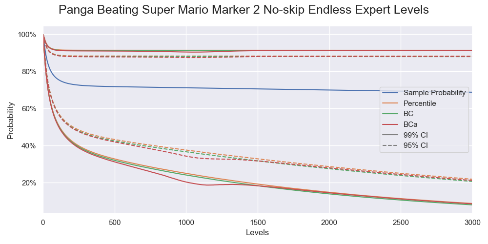
The confidence intervals calculated by the three bootstrap methods.
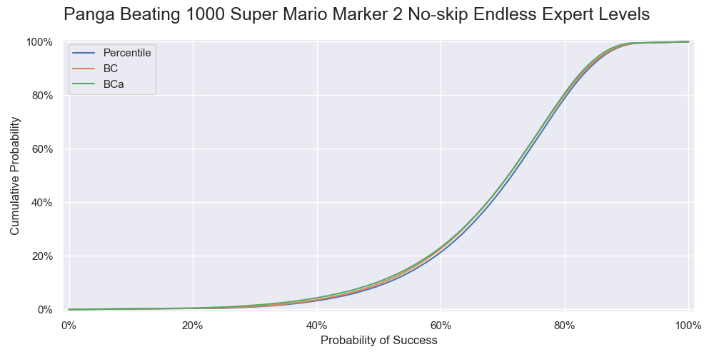
The cumulative distributions of the success rate of beating 1000 levels calculated by the three bootstrap methods.
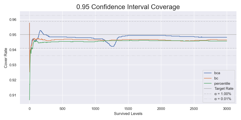
The coverages of 95% confidence intervals by 4000 simulations.
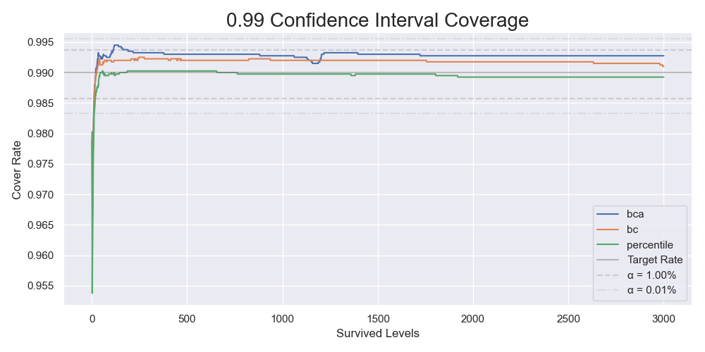
The coverages of 99% confidence intervals by 4000 simulations.
The same issue showed up again. In comparison, the BC bootstrap performed better than the BCa bootstrap. It gave similar results most of the time but without instability. Combining it with the result from the previous section that the non-parametric resampling process approximated the original sampling process well, we can conclude that the parametric BC bootstrap is the way to go. We have just come full circle.
Result
Panga did better in this larger set of samples than the subset in part 1. He gained 0.287 lives on average after beating a level. Below is the results. As a reminder, the inference used here is frequentist. The probabilities of the confidence intervals and cumulative probability refer to the corresponding (hypothetical) long-run frequencies of those being true for the same sampling and estimation procedure.
| Levels | Probability | 95% CI | 99% CI |
|---|---|---|---|
| 1000 | 71.2% | [36.7%, 88.1%] | [24.7%, 91.3%] |
| 2000 | 70% | [27.6%, 88.1%] | [14.4%, 91.3%] |
| 3000 | 68.8% | [20.7%, 88%] | [8.41%, 91.3%] |
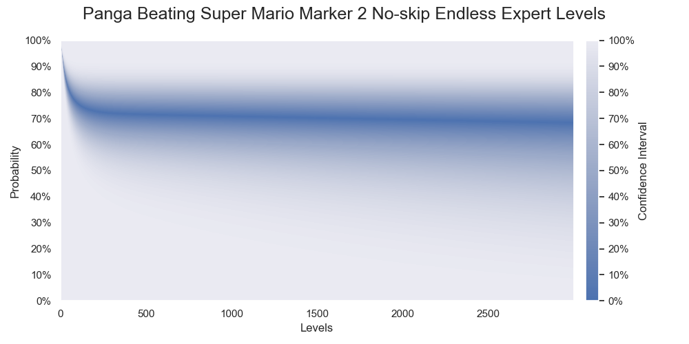
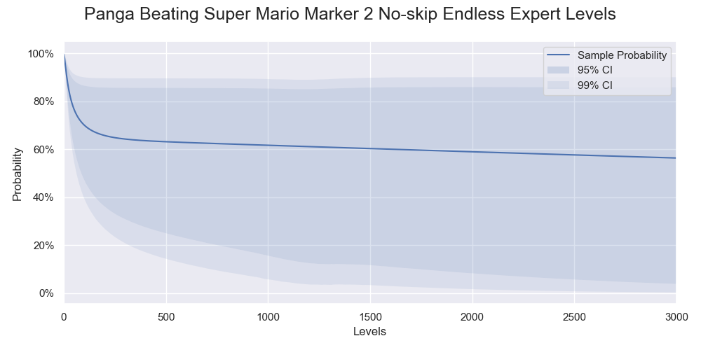
Probabilities of Panga successfully beating various numbers of levels. The darkest color denotes the medians of the probabilities.
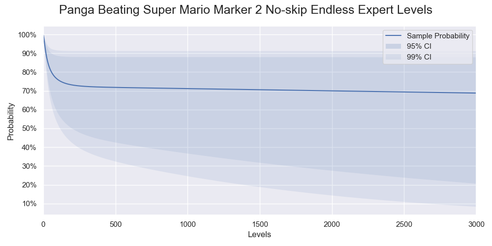
Probabilities of Panga successfully beating various numbers of levels. Only 95% and 99% confidence intervals are shown.
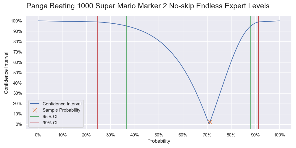
Probability of Panga successfully beating 1000 levels. It is a vertical slice of the level 1000 of the previous two graphs, and like a graph of the cumulative probability but with the 0% - 50% part being flipped upward.
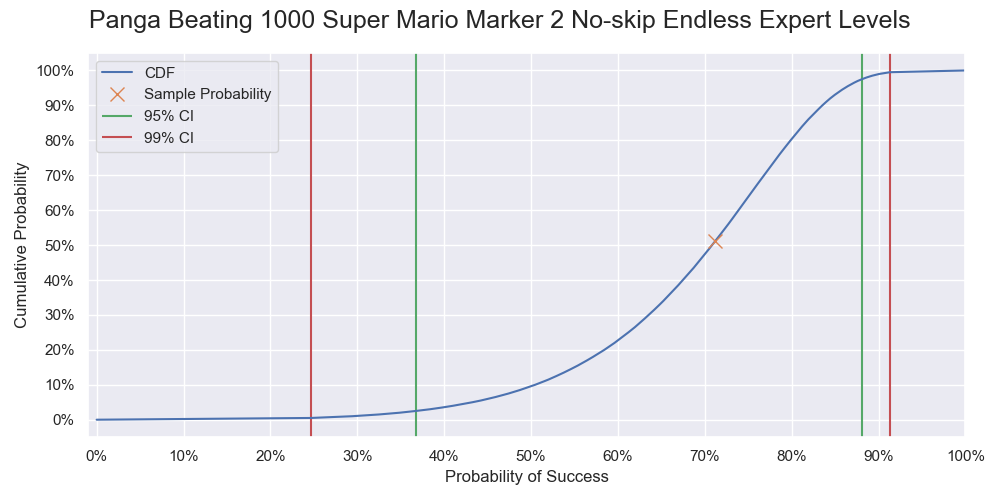
Cumulative probability of Panga successfully beating 1000 levels.
Compared to the result in part 1, the sample probabilities of beating 1000, 2000, and 3000 levels are 10% more. The upper confidence limits stay approximately the same while the bottom confidence limits shift upwards substantially. While most players struggle to beat 10 levels, Panga, being one of the best players in Super Mario Maker, only needs a few trials to have a decent chance to beat 1000 levels or even 2000 levels.
Conclusion
This time we have squeezed all information out of our precious samples. As of the time I am writing this, Panga's best run had already passed 1000 levels, ended at 1906 levels3. He is devoted to reaching 2000 levels. It means that we have more samples to reduce the uncertainty in our estimations. Besides, there are other interesting things to discuss in the part 3.
Bradley Efron & Balasubramanian Narasimhan (2020) The Automatic Construction of Bootstrap Confidence Intervals, Journal of Computational and Graphical Statistics, 29:3, 608-619, DOI: 10.1080/10618600.2020.1714633 ↩︎
Carpenter, J. and Bithell, J. (2000), Bootstrap confidence intervals: when, which, what? A practical guide for medical statisticians. Statist. Med., 19: 1141-1164. https://doi.org/10.1002/(SICI)1097-0258(20000515)19:9<1141::AID-SIM479>3.0.CO;2-F ↩︎
PangaeaPanga, This Run Got to ONE LIFE — Clearing 2000 EXPERT Levels (No-Skips) | S2 EP78 https://youtu.be/hvbGMohca94?t=1070 ↩︎