In part 2, we improved the estimation of Panga's success rates of beating the various numbers of levels without skipping by utilizing the samples with a better estimator. Meanwhile, he completed more levels in his pursuit of beating 2000 levels, and it means that we have more samples for our estimation.

New Data

With the new total of 2573 samples, far more than the previous 726 samples, the estimation will be significantly more precise. As expected, the distribution of the samples is similar to that before.

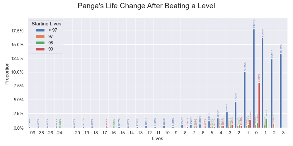
The overall sample distribution of Panga's life changes after beating a level. Values below 0.05% are visually enhanced.

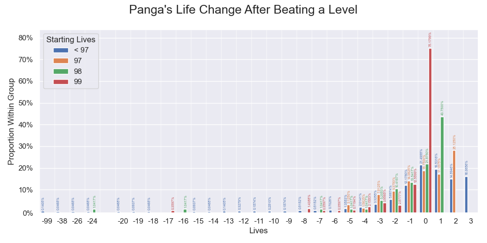
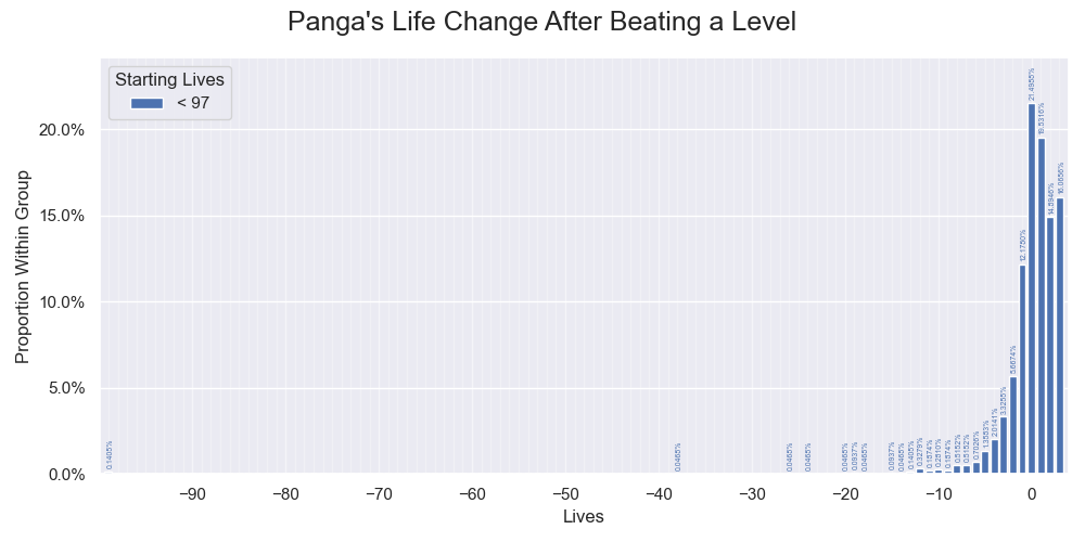
The within-group sample distribution of Panga's life changes after beating a level. Values below 0.05% are visually enhanced.

Panga's best run tragically ended by a triple-triple shell jump level (performing three triple shell jumps) and reached 1906 levels. The level required him to spend more than 99 lives to beat. Encountering such a level was virtually a guaranteed end of a run for any player. His two subsequent runs also ended similarly by two triple shell jump levels.

Validation of the Assumption in Part 1

In part 1, we made the assumption

The player performs practically the same when their number of lives is from 1 to 96 or 97 to 99.

To roughly check the assumption, we will compare the life change probabilities by considering the uncertainty per each starting life. As shown in the following graphs, almost all values are either very close or within random variations. The remaining rare instances are still explainable by random chance. Comparing the uncensored values across all the graphs, the results are the same.

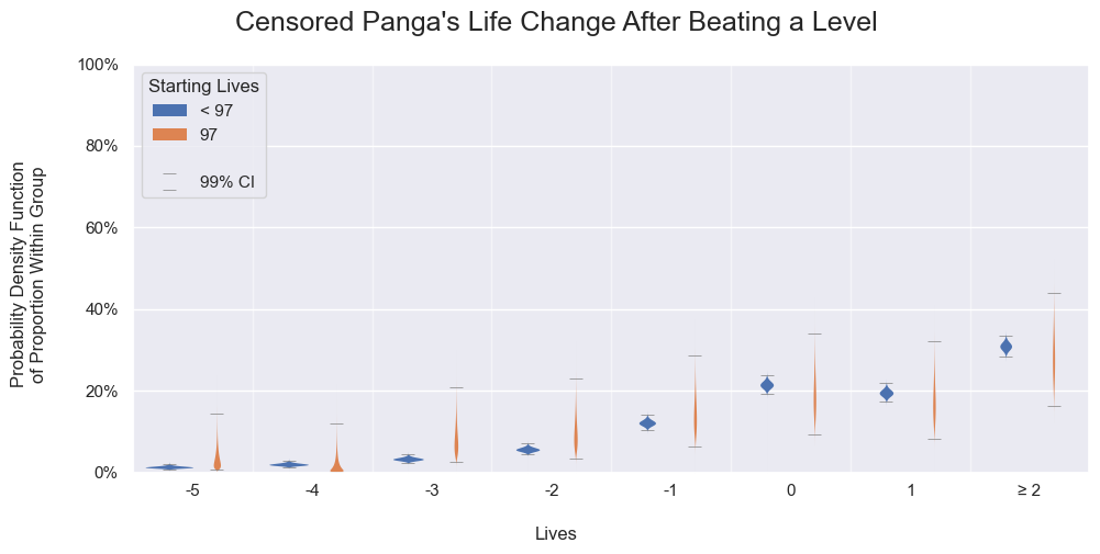
Panga's life change probabilities after beating a level for 97 starting lives or those below. Each probability density function is calculated independently by using the binomial proportion.

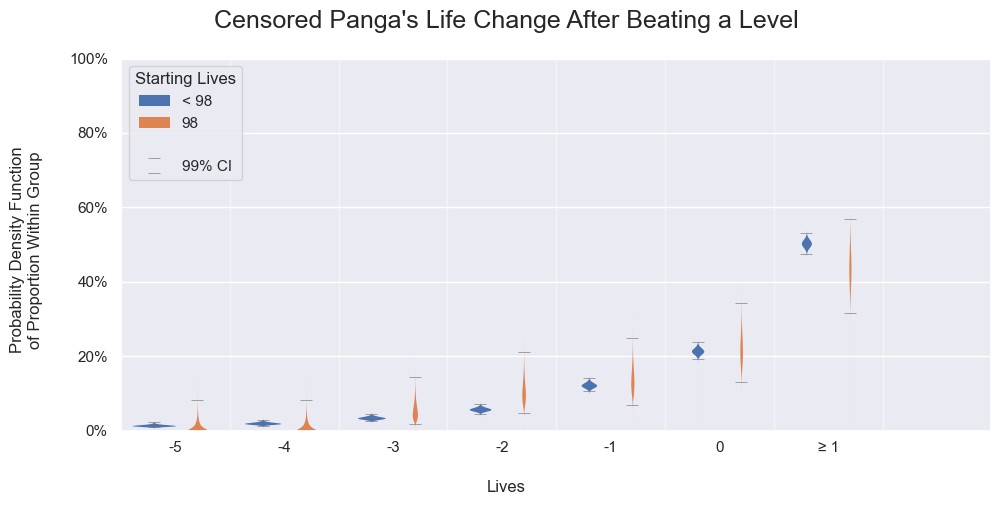
Panga's life change probabilities after beating a level for 98 starting lives or those below. Each probability density function is calculated independently by using the binomial proportion.

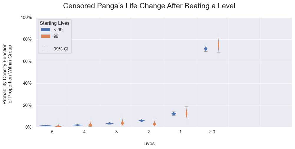
Panga's life change probabilities after beating a level for 99 starting lives or those below. Each probability density function is calculated independently by using the binomial proportion.

A complete and proper examination should be a hypothesis test like an equivalence test on more important combinations of the starting lives and life changes. People, even scientists, often misinterpret the significance of overlapping probabilities and error bars¹. I will leave the test for those who are interested. If you do, be aware of false discoveries you may encounter when checking too many combinations.

Result

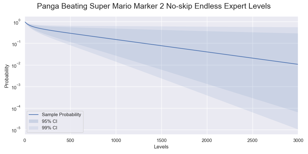
The sample probabilities and confidence intervals of Panga beating 1000, 2000, and 3000 levels plummet as the rare events surfaced. The sample probabilities hovered at 70% last time but become 15%, 4%, and 1% for the respective levels. The lower confidence limits are less than 3% to near impossible. The upper confidence limits drop from 91% to about 60%.

Levels	Probability	95% CI	99% CI
1000	14.9%	[2.68%, 48.5%]	[1.44%, 63%]
2000	3.97%	[0.131%, 36.9%]	[0.0391%, 59.2%]
3000	1.06%	[0.00633%, 29.2%]	[0.00104%, 55.8%]

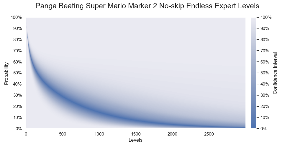
Probabilities of Panga successfully beating various numbers of levels. The darkest color denotes the medians of the probabilities.

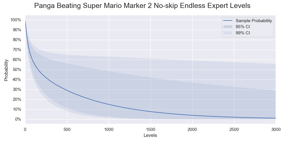
Probabilities of Panga successfully beating various numbers of levels. Only 95% and 99% confidence intervals are shown.

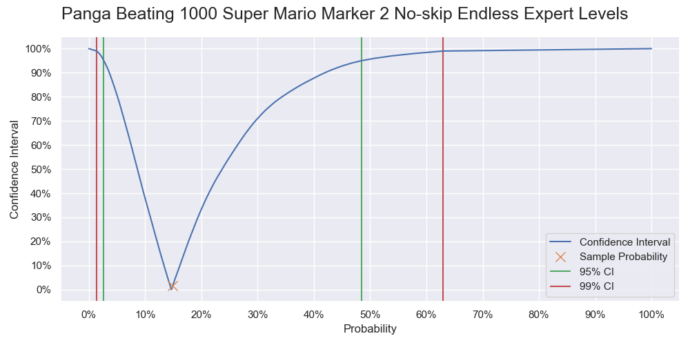
Probability of Panga successfully beating 1000 levels. It is a vertical slice of the level 1000 of the previous two graphs, and like a graph of the cumulative probability but with the 0% - 50% part being flipped upward.

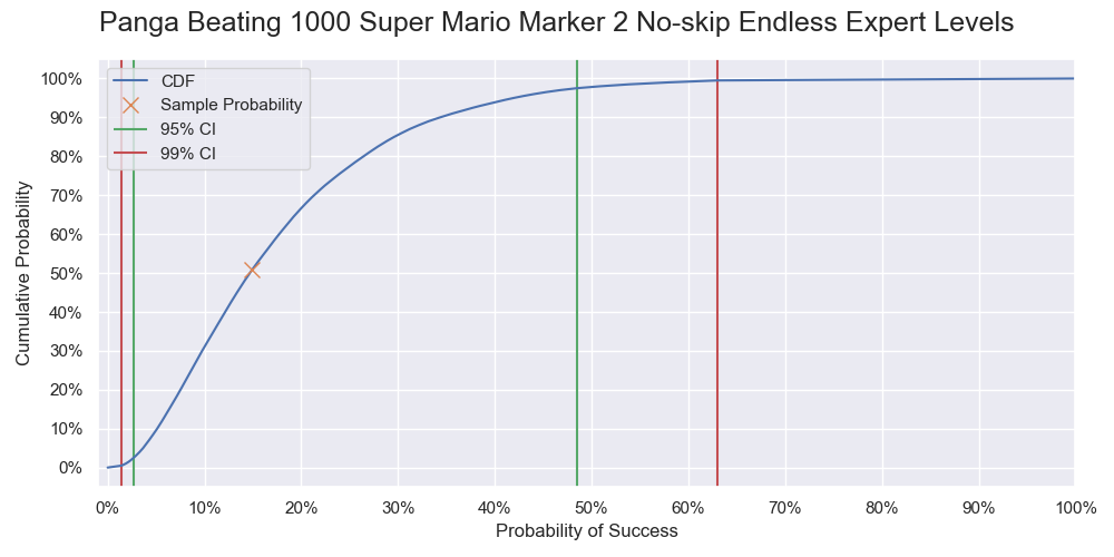
Cumulative probability of Panga successfully beating 1000 levels.

As a reminder, the inference used here is frequentist. The probabilities of the confidence intervals and cumulative probabilities refer to the corresponding (hypothetical) long-run frequencies that the sampling and estimation procedure are correct. For example, a 99% confidence interval means that 99% of such confidence intervals generated by the confidence procedure cover the true success rate. Whether an interval covers the true success rate is deterministic yes or no but is unknown to us.

Reaper Levels

Dodging run-ending levels are hard. It is like avoiding getting a one when you try throwing a dice many times. You may be able to throw 10 times, but if you keep throwing, you will eventually get a one. The exact probabilities of those happening are easy to calculate. Suppose that $ p $ is the probability of the outcome in an event, the probability of not having the outcome in $ n $ events is the complement of $ p $, raised to the power of $ n $:

$$ P(n) = (1 - p)^n $$

Let us only consider the sample probability of Panga encountering a run-ending level first for simplicity. It is 3 out of 2573 which is 0.117%. Plugging the number into the formula, we have the values shown in the following graph:

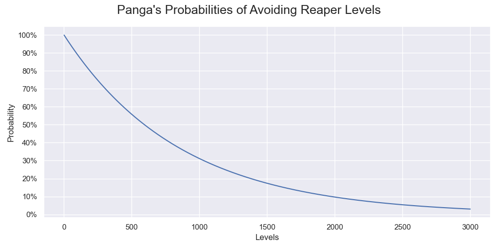
The probabilities of Panga doging a run-ending level when playing certain number of levels.

This kind of level alone is enough to bring the success rate of beating 1000 levels down to 31% and 2000 levels down to 9.7%.

The true probability of encountering a run-ending level is unknown as usual, so we should apply the formula to other possible values too. For instance, the upper 99% confidence limit of an encounter is 0.460%. It greatly lowers the success rate of beating 1000 and 2000 levels to 0.99% and 0.0099% respectively.

Precision

The estimations sometimes can be off very much as shown in part 2 and here. The estimated Panga's success rate of beating 1000 levels was previously 61.6% but is 14.9% here. The estimated success rate is sensitive to small errors in the estimated probabilities of encountering some levels, like the reaper levels. Recalls that we calculated the estimated success rate by multiplying the state vector to the transition matrix thousands of times. A small error accumulated into a huge error in the final estimation. Randomness was the first source of the error. Discreteness in the sample space, which was the probability of encountering a level causing a certain life change, was the second source. Such a sample probability could only be one of the finitely many values regardless of random chance. It might be $ \frac{1}{2573} $, $ \frac{2}{2573} $, $ \frac{3}{2573} $, or so on, but never $ \frac{0.5}{2573} $. The resolution might not be enough.

To illustrate the effect, we add one sample of each life change to the existing 2573 samples and calculate the corresponding rates:

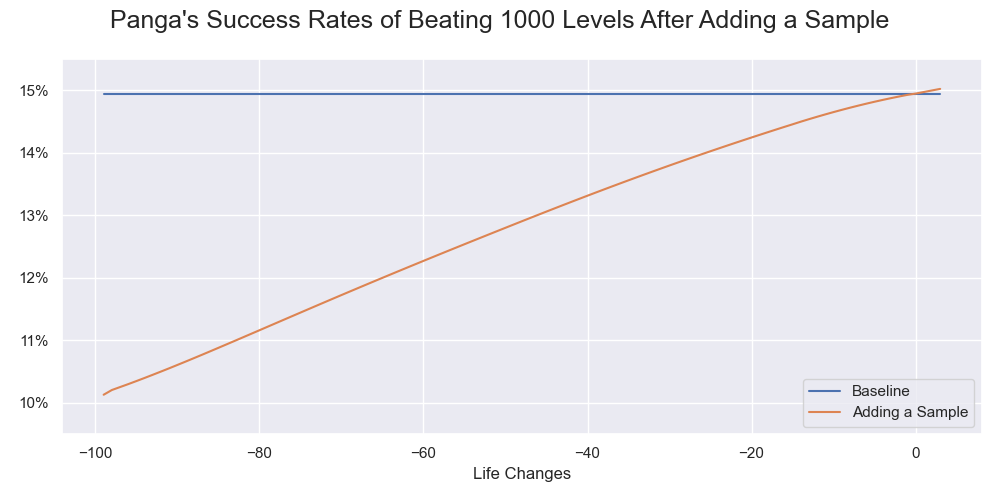
Panga's success rates of beating 1000 levels after adding a sample of various life changes.

The original sample success rate is about 15%. Adding a sample with a small life change does not affect the rate much. However, when the life loss increases, the difference grows substantially. At the extreme, it drops from 15% to 10%.

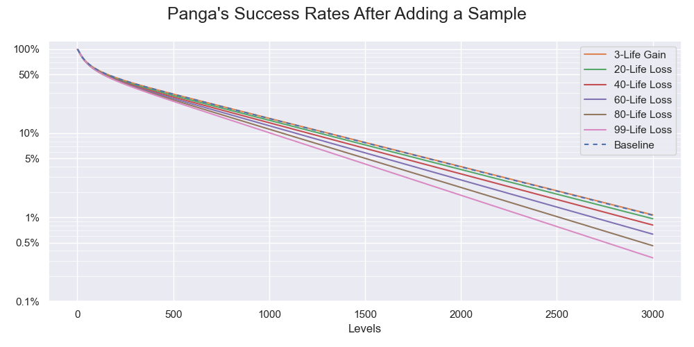
Panga's success rates of beating various numbers of levels after adding a sample of various life changes in a semi-log scale. The spaces between the lines denoting the success rates increase as the level of greater life loss is more impactful to the estimations.

The effect grows as the number of levels increases. At 1000 levels, the rate after adding a 99-life loss sample drops from 15% to 10%, which is one-third of 15%. At 3000 levels, it drops from 1% to 0.3%, which is two-thirds of 1%. In short, the estimations are sensitive to the discreteness and the randomness of some measurements. When everything compounds, they seriously affect the precision of our estimations.

What about the confidence intervals? Can they rescue us? The answer is "kind of". They help by stating intervals instead of point estimations but not in the way we demand. There is only one basic property of a confidence interval. Its construction procedure needs to generate intervals covering the true value with the specified rate in long run. The closeness between the ends of the intervals and the true value is not a concern, although some confidence intervals handle it somewhat nicely. The confidence interval calculated by Z-score for normal distributions is an example. If precision is a concern, it is better to directly estimate the precision, use an appropriate confidence procedure, or use other intervals, e.g. Bayesian credible intervals. Bayesian is another popular inference besides frequentist. When a credible interval says that the probability of a value falls into the interval, it means the probability among all possible parameters. That is what people usually have in mind. Credible intervals operate on likelihoods, so they are more connected to precision.

Despite all these, bootstraps are generally quite good at reflecting precision when there are sufficient samples. They have some Bayesian properties²³ and so produce intervals approximating credible intervals with a caveat. In "The Bayesian Bootstrap"², just as Rubin (1981) stated:

... is it reasonable to use a model specification that effectively assumes all possible distinct values of X have been observed? Both the BB and the bootstrap operate under this assumption. In some cases inferences may be insensitive to this assumption but not always. (p. 133)

We happened to encounter the perfect example in part 1, having no samples on the most influential non-zero parameter. However, this time we have samples for the 99-life loss. Even though we have no samples for other very large life losses, it should be fine. The distributions of the samples clearly show right-censored bell shapes. Extrapolating the trend to very large life losses indicates that the true probabilities are likely to be vanishingly small. They are different from the special 99 life-loss, which includes all even harder levels. Our new confidence interval now can reflect the precision.

The within-group sample distribution of Panga's life changes after beating a level with a start lives less than 97 in linear scales. The distribution shows a right-censored bell shape. Encountering a level causing a huge life loss other than 99 lives should be vanishingly rare.

To Infinity

The graph of the sample and confidence intervals of Panga's success rate of beating various levels looks suspiciously like exponential decays. Plotting it with a log scale on the y-axis reveals the long-term trend of the success rate, which is linear in a log scale.

Probabilities of Panga successfully beating various numbers of levels in a log scale. The decays are exponential and so linear in log scale.

It suggests the following asymptotic behaviors. Let

$ P(k) $ be the probability of beating $ k $ levels,
$ a $, $ b $ be some constants,
$ \lambda $ be the constant decay rate,

and with

$ \sim $ denoting "is asymptotically equivalent to",
$ \to $ denoting "tends to",
$ ak+b $ being the linear relationship.

We have

$$ \begin{aligned} P(k) &\sim e^{ak+b} \\ P(k+1) &\sim \lambda P(k) \quad \text{as } k \to \infty \\ \end{aligned} $$

The constant decay rate comes from a deeper cause. In part 1, we learnt that by formulating the problem as a Markov process, we could calculate $ P(k+1) $ from the state vector $ \vec s_k $ and transition matrix $ \mathbf T_{100\times100} $:

$$ \begin{aligned} \vec s_k &= \begin{bmatrix} P_s(k,\textcolor{red}{♥}=0) & P_s(k,\textcolor{red}{♥}=1) & \ldots & P_s(k,\textcolor{red}{♥}=99) \end{bmatrix} \\ \\ \mathbf T &= \begin{bmatrix} 1 & 0 & \ldots & 0 \\ P_t(\textcolor{red}{♥}=1,\Delta\textcolor{red}{♥}=-1) & P_t(\textcolor{red}{♥}=1,\Delta\textcolor{red}{♥}=0) & \ldots & P_t(\textcolor{red}{♥}=1,\Delta\textcolor{red}{♥}=98) \\ \vdots & \vdots & \ddots & \vdots \\ P_t(\textcolor{red}{♥}=99,\Delta\textcolor{red}{♥}=-99) & P_t(\textcolor{red}{♥}=99,\Delta\textcolor{red}{♥}=-98) & \ldots & P_t(\textcolor{red}{♥}=99,\Delta\textcolor{red}{♥}=0) \\ \end{bmatrix} \\ \\ \vec s_{k+1} &= \vec s_k \mathbf T \\ \\ P(k) &= 1 - P_s(k,\textcolor{red}{♥}=0) \\ &= \sum_{\textcolor{red}{♥}=1}^{99} P_s(k,\textcolor{red}{♥}) \end{aligned} $$

Partitioning the state vector gives the non-absorbing state (survival state) vector $ \vec r $ and the transition matrix gives the corresponding transition matrix $ \mathbf U_{99\times99} $:

$$ \begin{aligned} \vec s_{k} &= \begin{bmatrix} P_s(k,\textcolor{red}{♥}=0) & \vec r_k \end{bmatrix} \\ \mathbf T &= \left[ \begin{array}{c|c} 1 & \begin{matrix} 0 & \ldots & 0 \end{matrix} \\ \hline \begin{matrix} P_t(\textcolor{red}{♥}=1,\Delta\textcolor{red}{♥}=-1) \\ \vdots \\ P_t(\textcolor{red}{♥}=99,\Delta\textcolor{red}{♥}=-99) \end{matrix} & \Large \mathbf U \end{array} \right] \end{aligned} $$

Then we have:

$$ \begin{align} P(k) &= \sum_{i=1}^{99} r_{k,i} \notag \\ \vec r_{k+1} &= \vec r_k \mathbf U \label{eq1} \end{align} $$

The asymptotic process that a state is similar to its previous state causes exponential decay of the success rate:

$$ \begin{aligned} \vec r_{k+1} &\sim \lambda \vec r_k \quad \text{as } k \to \infty \\ P(k+1) &= \sum_{i=1}^{99} r_{k+1,i} \\ &\sim \sum_{i=1}^{99} \lambda r_{k,i} \\ &= \lambda P(k) \end{aligned} $$

A simple way to calculate the decay rate is to iterate equation $ \ref{eq1} $ until the value converges. The decay rate quickly converges to 99.87%.

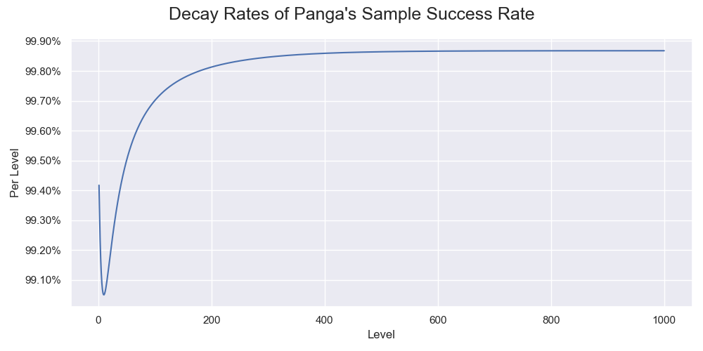
The decay rate of Panga's sample success rate in each iteration. It settles down at about 600 levels.

There is another interesting but slightly more complicated way to calculate the decay rate. $ \vec r_k $ are similar to each other and differ by a scale. If we normalize it, take the limit, and substitute it into $ \ref {eq1} $, we have a new equation:

$$ \vec r \mathbf U = \lambda \vec r $$

where

$$ \vec r = \lim_{k \to \infty}\frac{\vec r_{k}}{\sum_{i=1}^{99} r_{k,i}} $$

$ \vec r $ is an eigenvector of $ \mathbf U $ and $ \lambda $ is the corresponding eigenvalue. The equation means that when the vector multiplies the matrix, the result is the same as it multiplying with a constant. Such an equation is so common in science and engineering that most linear algebra software provides direct functionalities to solve it. However, the complication is after that. There are as many pairs of eigenvector and eigenvalue as the dimension of the matrix, which is 99 pairs here. For Panga's transition matrix, there is one sensible pair that

has a real eigenvector,
all elements in the eigenvector and the eigenvalue have the same sign.

Here, we only need to pick the pair of eigenvector and eigenvalue with all the elements being positive and the eigenvalue being less than one after normalization. Either way gives us the same solution.

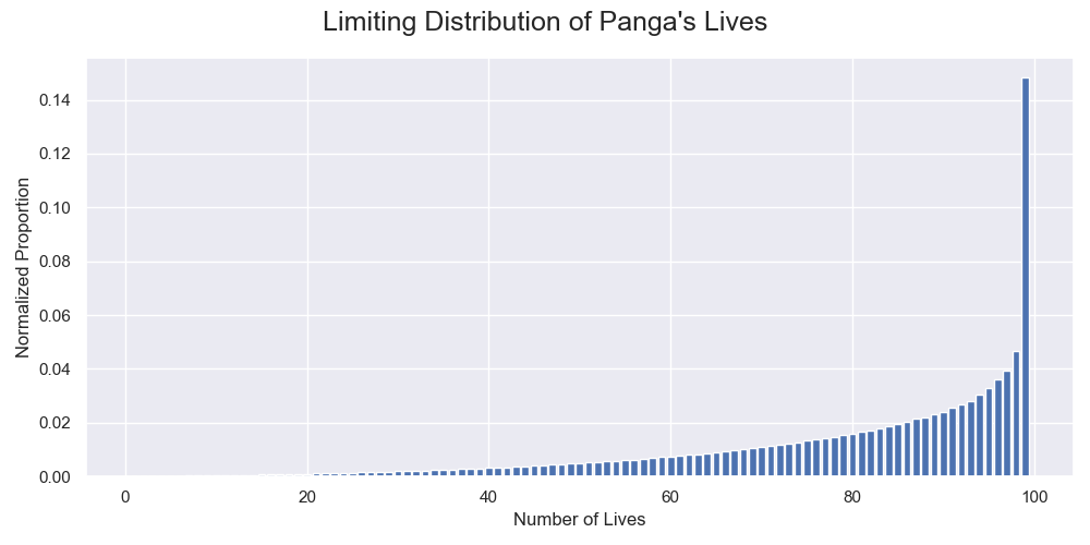
The normalized limiting distribution of Panga's lives $ \vec r $ after beating a level. Having a healthy amount of lives was one of his advantages.

Conclsuion

With the new samples, we could better validate the assumption we made before that the player performs practically the same regardless of their starting lives and improve the estimation of Panga's success rate. Our analysis revealed the key to performing well in the no-skip endless challenge other than being generally good at the game. Because Nintendo's level rating system is imprecise for freshly uploaded levels made by and played by other top players, you must prepare for those levels too. We also experienced a perfect example of the limitation of bootstraps. They did not give confidence intervals that had the Bayesian properties and fell back to the minimal frequentist interpretation when there were insufficient samples for sensitive parameters. Perhaps in the future, we will try a Bayesian inference.

Krzywinski, M., Altman, N. Error bars. Nat Methods10, 921–922 (2013). https://doi.org/10.1038/nmeth.2659 ↩︎
Donald B. Rubin. "The Bayesian Bootstrap." Ann. Statist. 9 (1) 130 - 134, January, 1981. https://doi.org/10.1214/aos/1176345338 ↩︎
Trevor Hastie, Robert Tibshirani, Jerome Friedman. The Elements of Statistical Learning: Data Mining, Inference, and Prediction. Second Edition, February 2009. ↩︎

Endless Expert Levels Without Skipping in SMM2 - Part 3